Distributed Training Techniques for LLM

Bottlenecks of Single-Machine LLM Training

1. LLMs are getting larger, and single-machine GPU memory is insufficient.

2. Training speed is insufficient.

Directions for Distributed Parallel Training

LLMs can be distributed and split from three perspectives:

1. Data Parallelism (most widely applied)
2. Model Parallelism / Pipeline Parallelism / Layer-wise Parallelism (different names)
3. Tensor Parallelism / Intra-layer Parallelism (different names)

All three parallel approaches can even be applied simultaneously to maximize GPU memory utilization and accelerate training.

Data Parallelism

The original data is divided into different disjoint subsets, and different computing devices process the sub-training sets separately. Since each computing device independently stores a complete copy of the model, the gradients obtained from backpropagation on each device need to be aggregated and averaged. In the Transformer architecture, the forward and backward propagation of each operator only depends on a single data sample, not the entire training batch. Therefore, no matter how the data is partitioned, implementing parallelism does not affect the gradient computation logic.

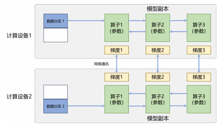
This parallel approach does not involve synchronization issues between computing devices and achieves the highest speedup ratio. However, each device needs to retain the complete model parameters, so it is still not practical for training large LLMs.

Communication volume analysis:

Input phase: $(N - 1) \frac{\phi}{N}$

Pipeline Parallelism / Layer-wise Parallelism / Model Parallelism

If a single GPU cannot store the entire model's parameters, why not split the model as well? Different computing devices store different layers of the model, which can effectively reduce the model storage footprint on a single device.

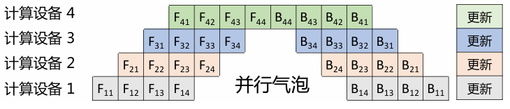
The idea of pipeline parallelism originates from CPUs, and it also encounters the same parallel bubble problem found in CPUs. During the warm-up phase, downstream computing devices need to wait for results from upstream computing devices. The resource waste caused by this waiting is called a parallel bubble.

Looking closely at the figure above, when computing device 4 performs backpropagation $B_{44}$, it cannot perform forward propagation $F_{54}$ (not shown in the figure). This is the parallel bubble caused by a single computing device being responsible for both forward and backward propagation simultaneously.

Megatron proposed a solution that separates forward and backward propagation, reducing parallel bubbles. However, the process is somewhat difficult to understand, so I will leave this as a topic for future exploration.

Tensor Parallelism

The idea of tensor parallelism is to split individual operators, i.e., intra-layer splitting and parallelism. Since operators vary greatly, the feasibility of splitting and the implementation approach need to be analyzed individually, which is quite troublesome and not as general as pipeline parallelism.

Analyzing only the Transformer architecture, the main operators include: Embedding, MatMul, and Cross Entropy Loss.

If we want to split Embedding, we can only cut along the word_size dimension and distribute the pieces across different computing devices.

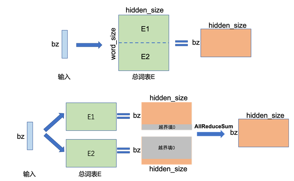
If the entire Embedding size is $640000*5120$, using FP32 representation would occupy $640000 * 5120 * 4 / 1024 / 1024 = 1250MB$. The gradients from backpropagation also occupy $1250MB$. If an Adam-type optimizer is used, the first-order momentum and second-order momentum each occupy another $1250MB$, totaling $5GB$. If we split the Embedding into two identical parts along the word_size dimension, each device only occupies $2.5GB$, which is quite cost-effective.

Since the Embedding is split across two different devices, using it becomes troublesome. It needs to be processed on each device and then aggregated, which is the AllReduceSum shown in the figure.

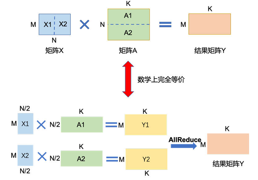
If we want to split the matrix multiplication MatMul, we can only use the block matrix method from linear algebra (it turns out that block matrix knowledge actually has practical applications :)).

Distributed Communication Architecture

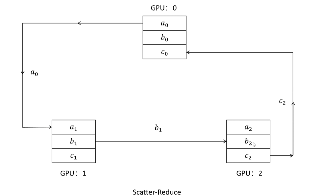
The three approaches mentioned above only analyze from which perspectives data or models can be split, and then results are aggregated through communication. Here, we delve deeper into the specific distributed communication methods, specifically the decentralized architecture.

Distributed communication primitives:

• Scatter: The master node partitions the data and distributes it to other specified nodes.
• Broadcast: The master node sends its own data to other nodes in the cluster.
• Reduce: A general term for a series of simple operations that aggregate computation results from different nodes.
• AllReduce: Applies the same Reduce operation on all nodes.
• Gather: Collects data from multiple nodes onto a single node. Gather can be understood as the reverse of Scatter.
• AllGather: Collects data from all other nodes on every node.
• ReduceScatter: Splits the tensor on each node into multiple blocks, with each block assigned to a different node.

Decentralized distributed architecture:

Distributed communication acceleration strategies:

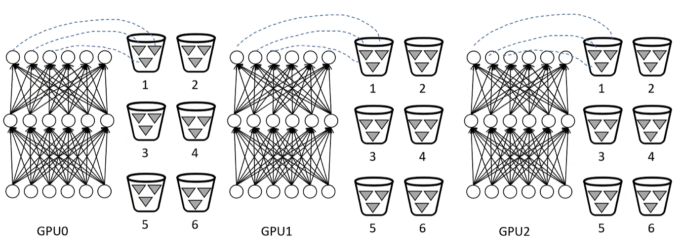
By setting up parameter listeners and storing parameter gradients in buckets, the communication speed of gradient parameters is greatly improved (the same principle as buffered I/O in operating systems).

Industrial Implementations

NVIDIA's open-source Megatron and Microsoft's open-source DeepSpeed both provide distributed training capabilities. The former focuses more on tensor parallelism, while the latter focuses more on data parallelism and model parallelism.

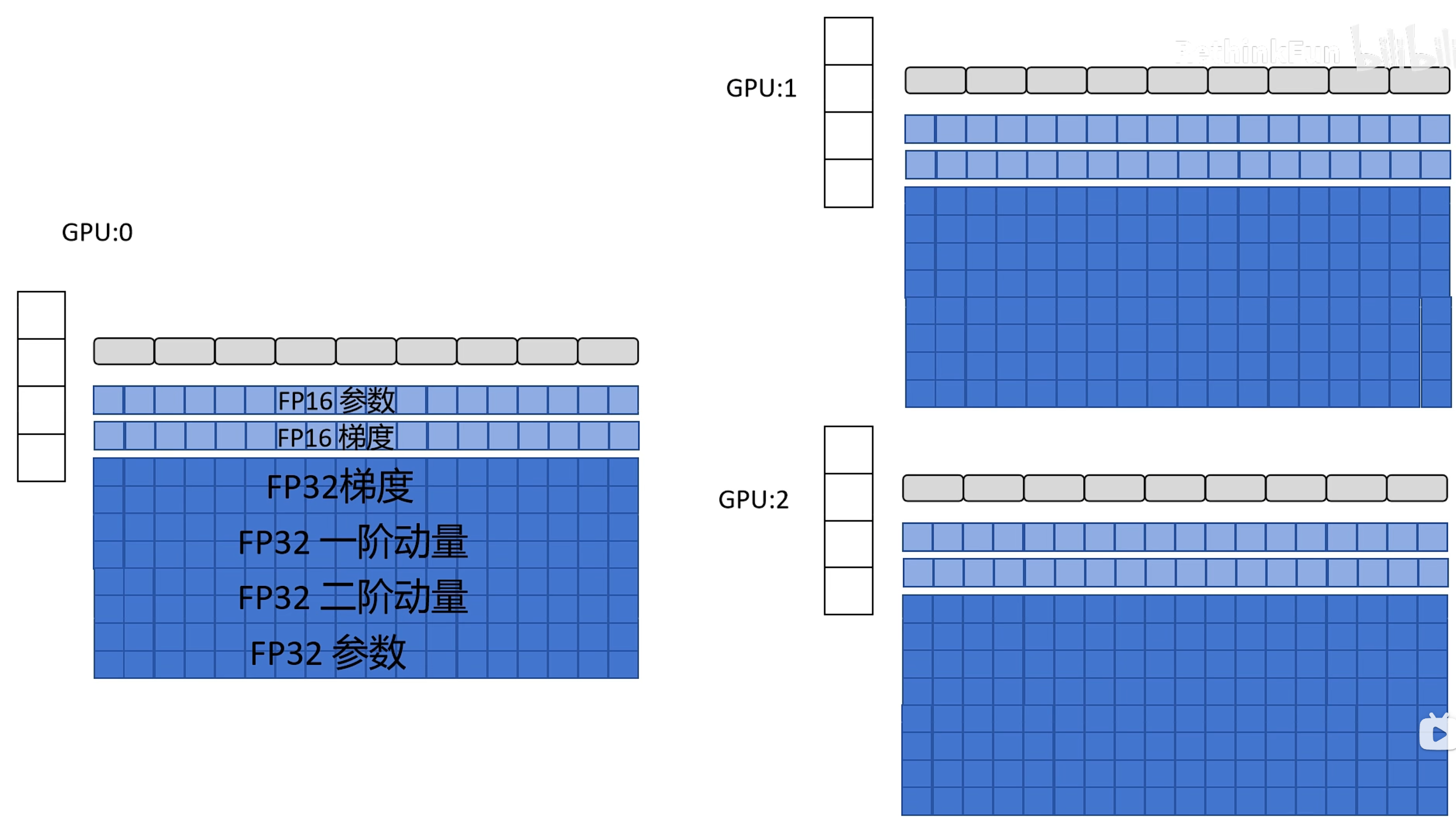
As shown in the figure, under mixed precision and Adam conditions, GPU memory usage consists of: FP16 representation of model parameters, FP16 representation of model gradients, full-precision FP32 model parameters, and full-precision FP32 gradients/first-order momentum/second-order momentum.

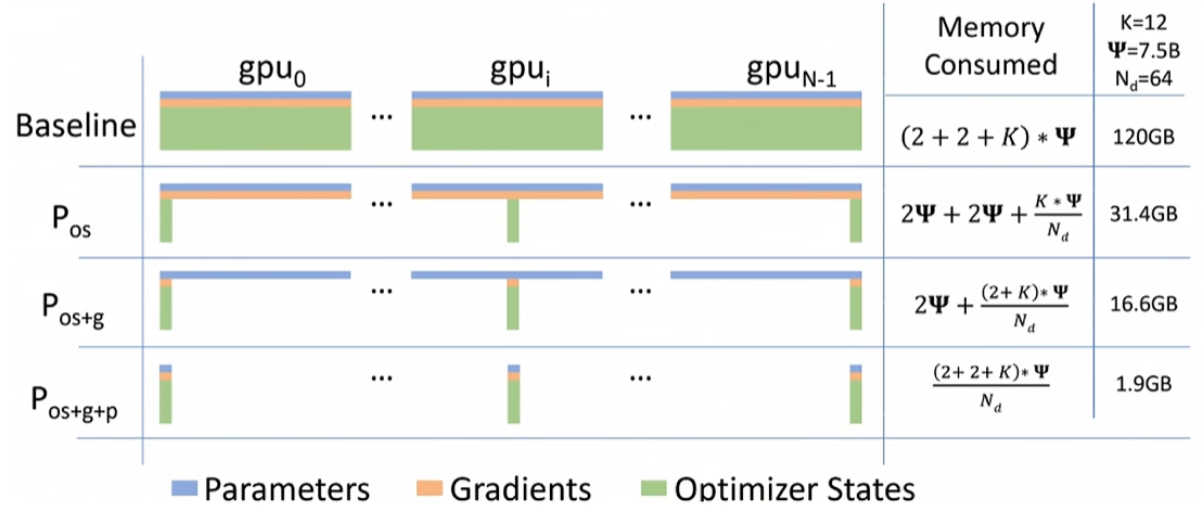
DeepSpeed provides three levels of parameter redundancy elimination. The GPU memory optimization at different levels is shown below:

DeepSpeed ZeRO-1

Zero optimizer parameter redundancy: Each computing device only retains the optimizer parameters for the portion of model parameters it is responsible for.

DeepSpeed ZeRO-2

Zero optimizer parameter + gradient redundancy: Since each device only updates the model parameters it is responsible for, it only needs to retain the gradients for its own model parameters.

During backpropagation, after $gpu_0$ and $gpu_1$ compute their gradients, they immediately send them to $gpu_3$ and release the GPU memory. Only $gpu_3$ computes the average of the total model gradients. The subsequent process of updating gradients for earlier model parameters is similar.

DeepSpeed ZeRO-3

Zero optimizer parameter + gradient + model parameter redundancy: Model parameters are also partitioned across different computing devices.

For example, during forward propagation, $gpu_1$ and $gpu_2$ do not have the parameters of the first layer (these are FP16 model parameters), so $gpu_0$ must broadcast the parameters to them. After the computation is complete, the GPU memory is immediately released.